Intergranular Strain

The intergranular strain concept enables hypoplasticity models to predict stiffness at very small strains, recent stress history and the effects of cyclic loading. The following features are predicted:

Elastic very small strain stiffness and its non-linear decrease with strain
Dependency of stiffness in the small strain range on loading direction, the effects of recent stress and strain history
Cyclic hysteresis and stress or strain accumulation during cyclic loading

The intergranular strain concept can be used in combination with both the sand and clay models. The parameters differ in detail (see below) but the model formulation is similar in the two cases. For detailed description of the intergranular strain concept calibration, see the following document. Brief description of the parameters is given below.

Model parameters

The intergranular strain concept uses five (six in clay hypoplasticity) material parameters additional to the parameters of the basic hypoplastic model. The parameters are:

$m_R$ (sand model) or $A_g$ and $n_g$ (clay model) - Parameters controlling the initial (very-small-strain) shear modulus upon 180° strain path reversal and in the initial loading
$m_T$ (sand model) or $m_{rat}$ (clay model) - Parameter controlling the initial shear modulus upon 90° strain path reversal
$R$ - The size of the elastic range (in the strain space)
$\beta_r$ and $\chi$ - Parameters controlling the rate of stiffness degradation with strain

The intergranular strain concept adopts one additional tensorial state variable denoted as intergranular strain. This state variable enables the model to keep track of the previous strain history.

Parameter $m_R$ (sand model) or $A_g$ and $n_g$ (clay model)

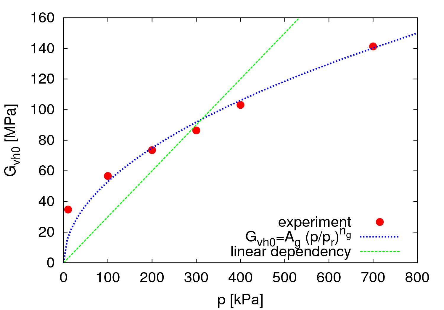
These two parameters affect the value of shear modulus at very small strains, as measured in shear wave propagation tests (for example, bender element tests). Clay model can be calibrated directly using \begin{equation} G_0=p_r A_g \left(\frac{p}{p_r}\right)^{n_g} \end{equation} the resulting curve of shear modulus at very small strain $G_0$ vs. the mean effective stress $p$ is shown in Figure 1.

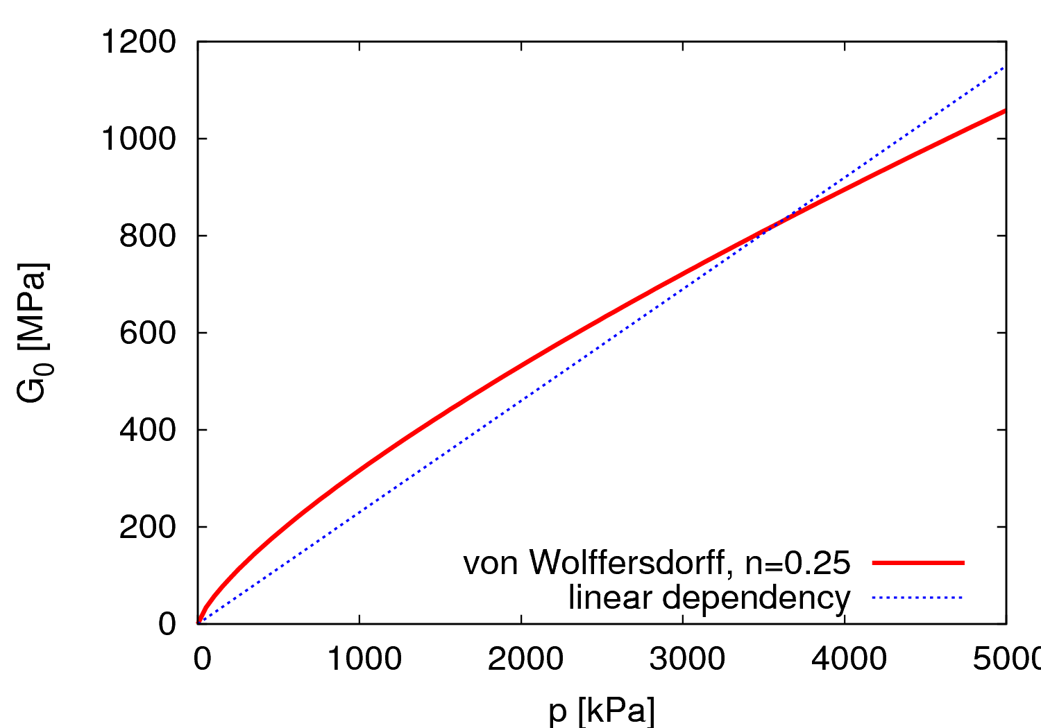
Figure 1: $G_0$ vs. p dependency for the intergranular strain concept used with the clay model

In the sand model, $m_R$ cannot be calibrated by a direct curve fitting. Instead, a single element simulation of the shear experiment is needed. The value of $G_0$ will be proportional to $p^{1-n}$, where $n$ is the basic sand model parameter. Example of $G_0$ vs. $p$ curve is in Figure 2.

Figure 2: $G_0$ vs. p dependency for the intergranular strain concept used with the sand model

Parameter $m_T$ (sand model) or $m_{rat}$ (clay model)

Parameters $m_T$ (sand model) or $m_{rat}$ (clay model) represent the $G_{90}/G_0$ ratio, where $G_{90}$ is the initial shear stiffness after 90° change of strain path direction. This parameter is problematic to calibrate using experimental data. Therefore, empirical estimation $m_{rat}=0.7$ (clay model) or $m_{T}=0.7m_{R}$ (sand model) is advocated.

Parameters $R$

Parameter $R$ represents the size of the elastic range, measured in the strain space. As a consequence, it affects the initial portion of the stiffness degradation curve, as shown in Figure 3.

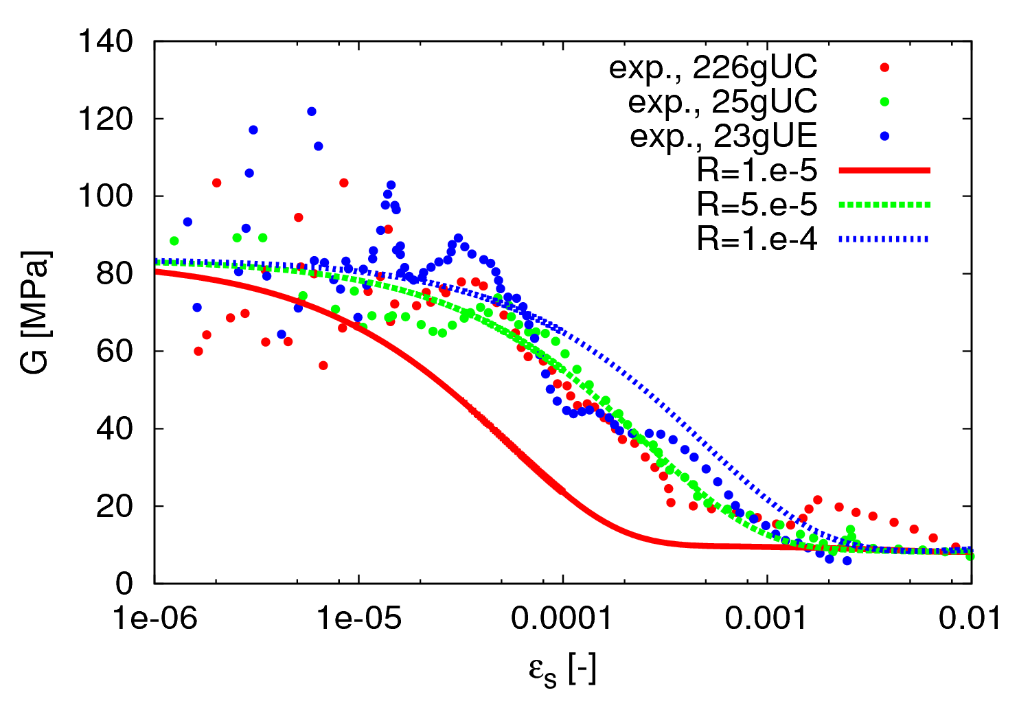
Figure 3: The effect of $R$ on the shear stiffness degradation curve in undrained triaxial test on clay

Parameters $\beta_r$ and $\chi$

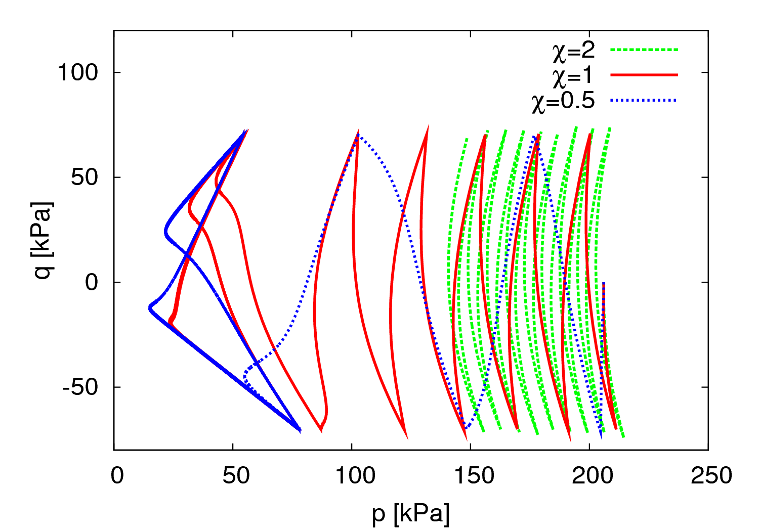
Parameters $\beta_r$ and $\chi$ control the rate of stiffness degradation curve. As shown in Figures 4 and 5, $\beta_r$ shifts the curve horisontally in the $G_0$ vs $\ln(\epsilon_s)$ space, whereas $\chi$ affects its slope.

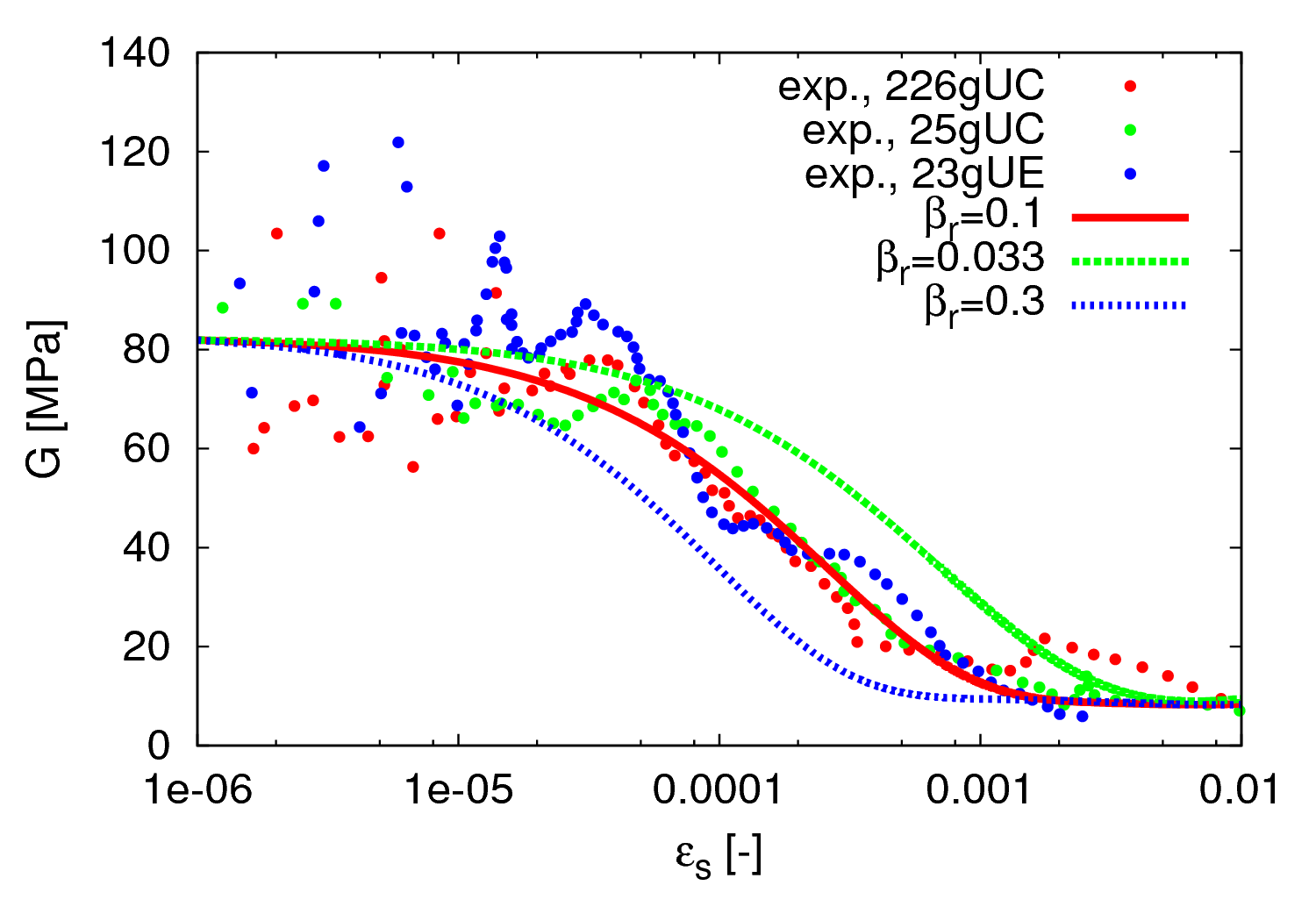
Figure 4: The effect of $\beta_r$ on the shear stiffness degradation curve in undrained triaxial test on clay

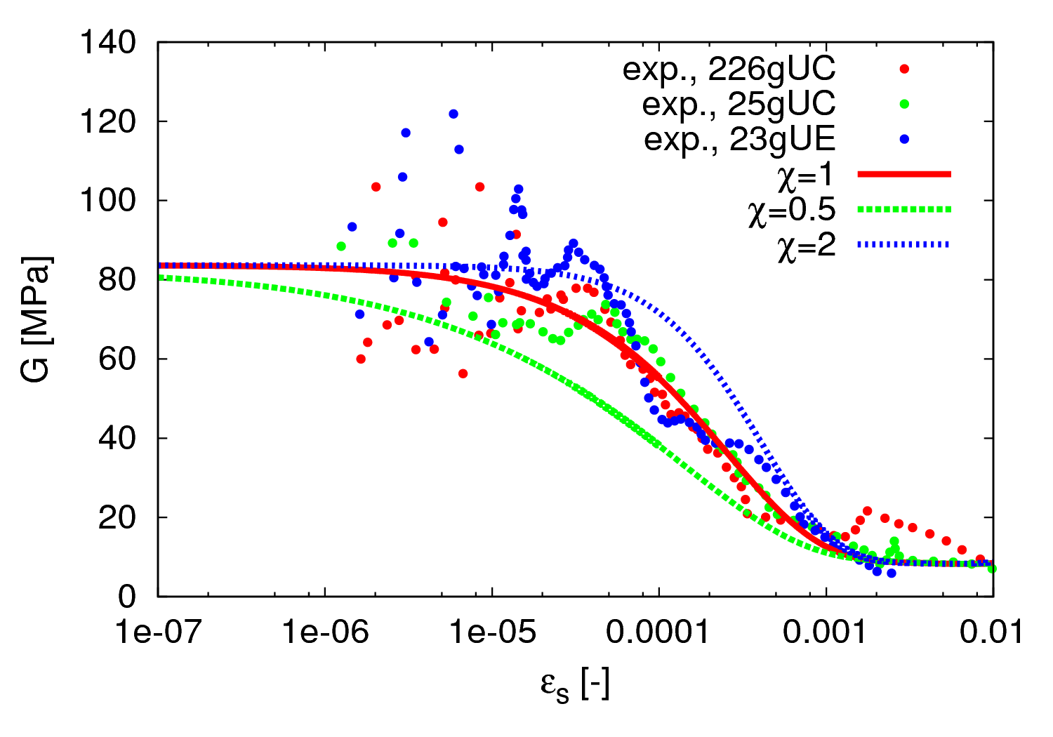
Figure 5: The effect of $\chi$ on the shear stiffness degradation curve in undrained triaxial test on clay

Calibration of the parameters using cyclic triaxial tests

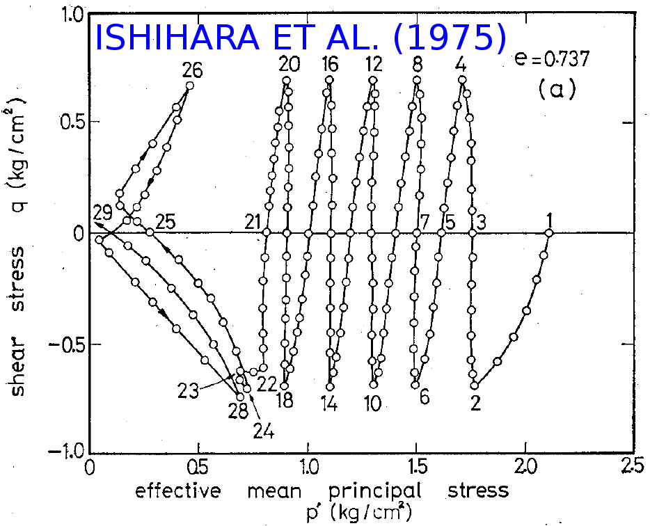
If the intergranular strain is to be used for predicting the cyclic soil response, the cyclic tests can also be used for the model parameter calibration. Example results on Toyoura sand by Ishihara et al. (1975) are shown in Figure 6.

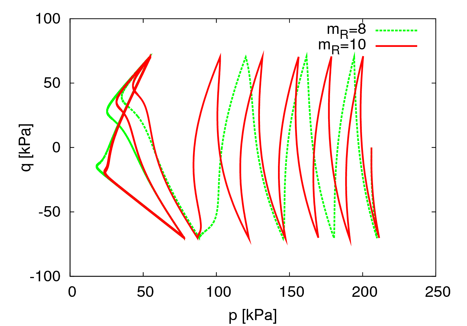
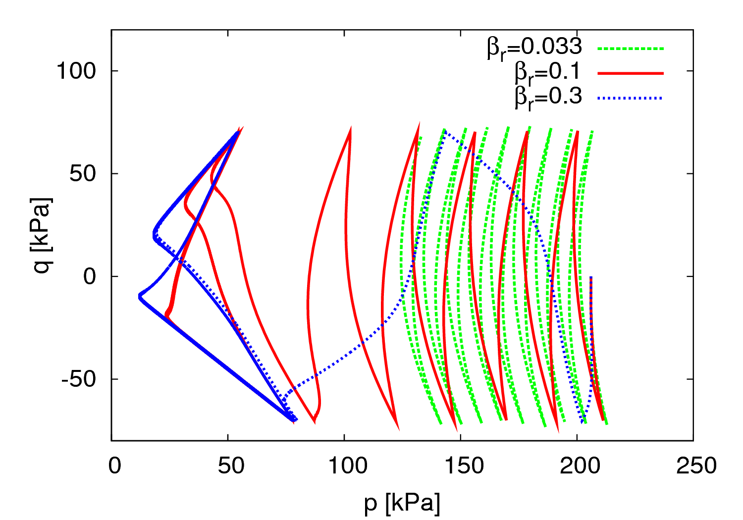
Figure 6: Cyclic drained triaxial test results on Toyoura sand (Ishihara et al., 1975)

The effect of the parameters $m_R$, $\beta_r$ and $\chi$ on the model predictions is plotted in Figures 7 to 9.

Figure 7: The effect of $m_R$ on the cyclic drained triaxial test predictions

Figure 8: The effect of $\beta_r$ on the cyclic drained triaxial test predictions

Figure 9: The effect of $\chi$ on the cyclic drained triaxial test predictions

It is clear from Figures 7 to 9 that the effect of $m_R$, $\beta_r$ and $\chi$ on the accumulation of strain due to cyclic loading is hard to distinguish. For this reason, the following calibration procedure is recommended:

Treat $R = 10^{−4}$ and $\chi = 1$ as material independent constants
Calibrate $m_R$ ($A_g$ and $n_g$ for the clay model) using bender element measurements (they are relatively easy to perform)
Set $m_T = 0.7m_R$ ($m_{rat} = 0.7$)
Control the cyclic behaviour using the parameter $\beta_r$ only.